
COINr is an open-source R package for building and analysing composite indicators, developed by the European Commission’s Joint Research Centre. The COINr package has many functionalities, and the full documentation can be found here. Here, a few highlights are given.
All of the highlights will be demonstrated on COINr’s inbuilt “ASEM data set”, which is a composite indicator created to measure international sustainable connectivity, and is based on the indexes found at the ASEM Sustainable Connectivity Portal.
We will begin by building this in COINr:
library(COINr)
##
## Attaching package: 'COINr'
## The following object is masked from 'package:stats':
##
##     aggregate
library(magrittr)
ASEM <- build_ASEM()
## -----------------
## Denominators detected - stored in .$Input$Denominators
## -----------------
## -----------------
## Indicator codes cross-checked and OK.
## -----------------
## Number of indicators = 49
## Number of units = 51
## Number of reference years of data = 1
## Years from 2018 to 2018
## Number of aggregation levels = 3 above indicator level.
## -----------------
## Aggregation level 1 with 8 aggregate groups: Physical, ConEcFin, Political, Instit, P2P, Environ, Social, SusEcFin
## Cross-check between metadata and framework = OK.
## Aggregation level 2 with 2 aggregate groups: Conn, Sust
## Cross-check between metadata and framework = OK.
## Aggregation level 3 with 1 aggregate groups: Index
## Cross-check between metadata and framework = OK.
## -----------------
## Missing data points detected = 65
## Missing data points imputed = 65, using method = indgroup_mean
Build with no limits
COINr has a rich set of tools for constructing composite indicators from raw indicator data. Unlike other composite indicator tools, COINr has very few limits. Construction features include:
- No limits on the number of indicators, units (i.e. countries/regions), or number of aggregation levels. Your composite indicator can be the size and shape you want it to be.
- Denomination by other indicators (including built in world denominators data set)
- Screening units by data requirements
- Imputation of missing data, by either:
- Global mean or median of indicator values
- Group mean or median of indicator values
- Mean or median within an aggregation group
- Expectation maximisation algorithm
- Normalisation by any of the following methods, either for all indicators or for each individually:
- Min max
- Z-score
- Linear scale
- Rank
- Borda
- Percentile rank
- Fraction of maximum indicator value
- Distance to a reference unit
- Distance to maximum indicator value
- Distance to indicator target
- Custom normalisation function
- Weighting using either:
- Equal weighting
- Manual weighting (including an interactive reweighting app)
- PCA weights
- Correlation-optimised weights
- Aggregation of indicators using any of the following for each aggregation level:
- Arithmetic weighted mean
- Geometric weighted mean
- Harmonic weighted mean
- Median
- Copeland method
- A custom aggregation function
All of these features are easily accessible via a harmonised “COINrverse” system, which is up next.
Live in the COINrverse (or not)
Many COINr functions can be used two ways: either as standalone functions which operate on a data frame (e.g. normalising a data frame of indicator data), or on a so-called COIN.
COINs are hierarchical lists, a bit like a folder system. In R they are sometimes called “lists of lists” or “nested lists”. A COIN contains all the data, parameters, methodological choices and results of a composite indicator. It has a structure something like this:
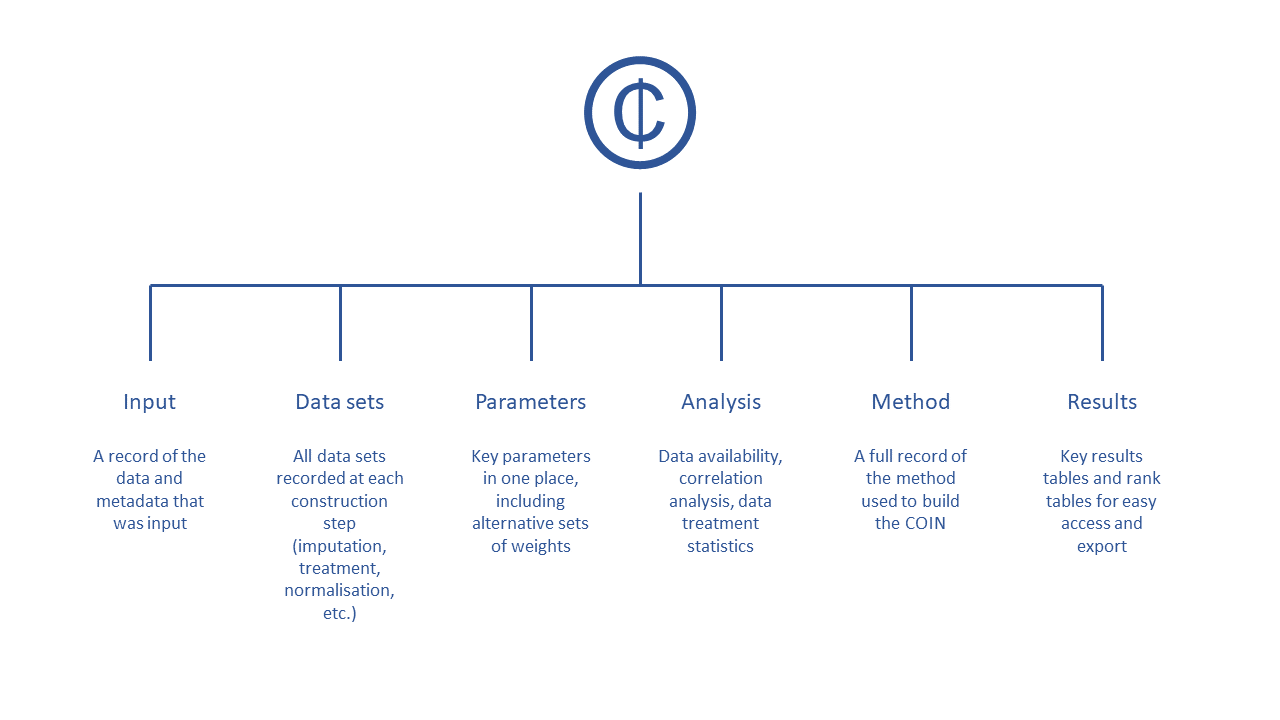
Inside a COIN
In short, a COIN contains everything relating to your composite indicator in a single “object”. There are at least three good reasons for this:
- A streamlined syntax because functions know where data and parameters are. Therefore, COINr operations typically follow a syntax of the form
COINobj <- COINr_function(COINobj, <methodological settings>), updating the COIN object with new results and data sets generated by the function. - It keeps things organised and avoids a workspace of dozens of variables.
- It keeps a record of methodological decisions - this allows results to be easily regenerated following “what if” experiments, such as removing or changing indicators and comparing alternative versions of the same index.
All the stats you could want
Hello stats:
getStats(ASEM, dset = "Aggregated", out2 = "list")$StatTable %>% reactable::reactable()
## Number of collinear indicators =  5
## Number of signficant negative indicator correlations =  396
## Number of indicators with high denominator correlations =  0
Easy plots
COINr provides many different types of plots, all accessible with simple functions. They follow a “plot first, adjust later” logic: because they are powered by the plotly and ggplot2 packages, they can be fine tuned using functions from these packages.
COINr plots include framework plots:
plotframework(ASEM)Indicator distribution plots:
plotIndDist(ASEM, type = "Violindot", icodes = "Physical")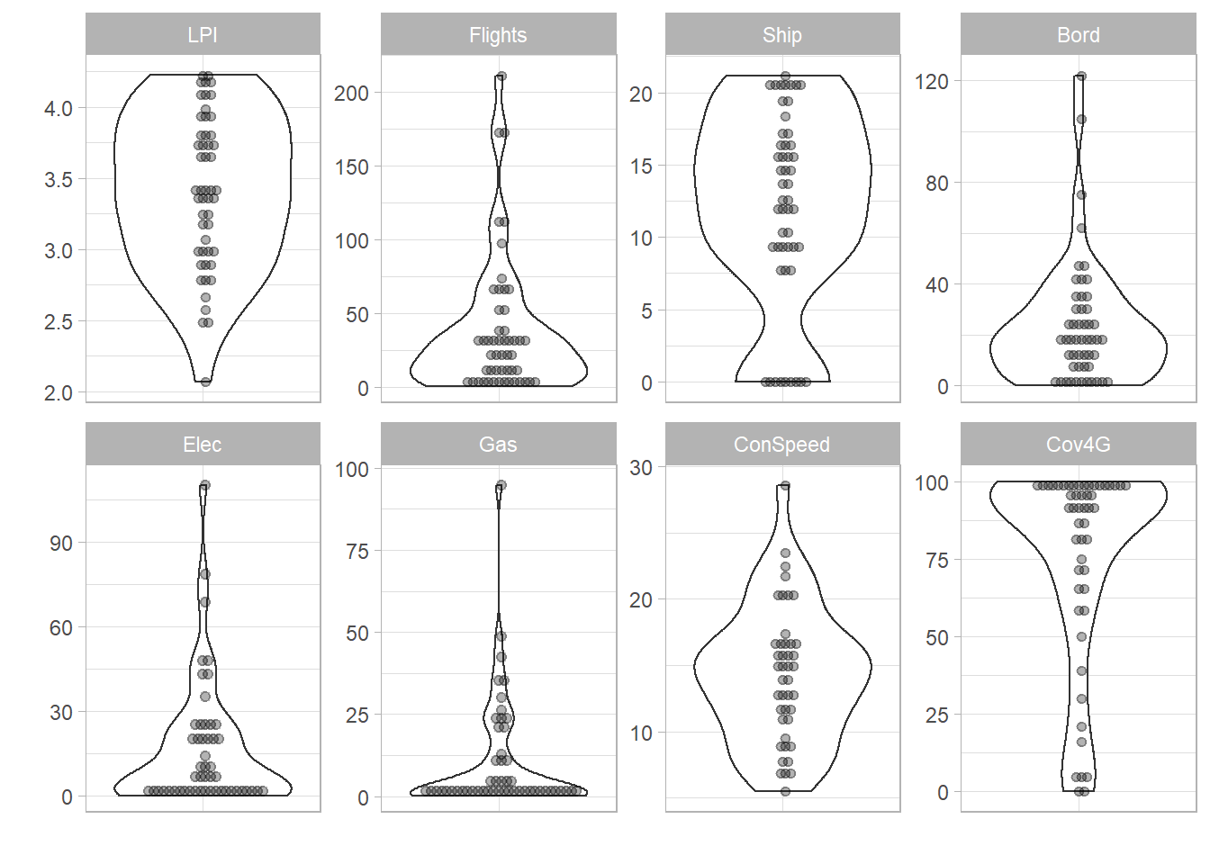
plotIndDist(ASEM, type = "Box", icodes = "Political")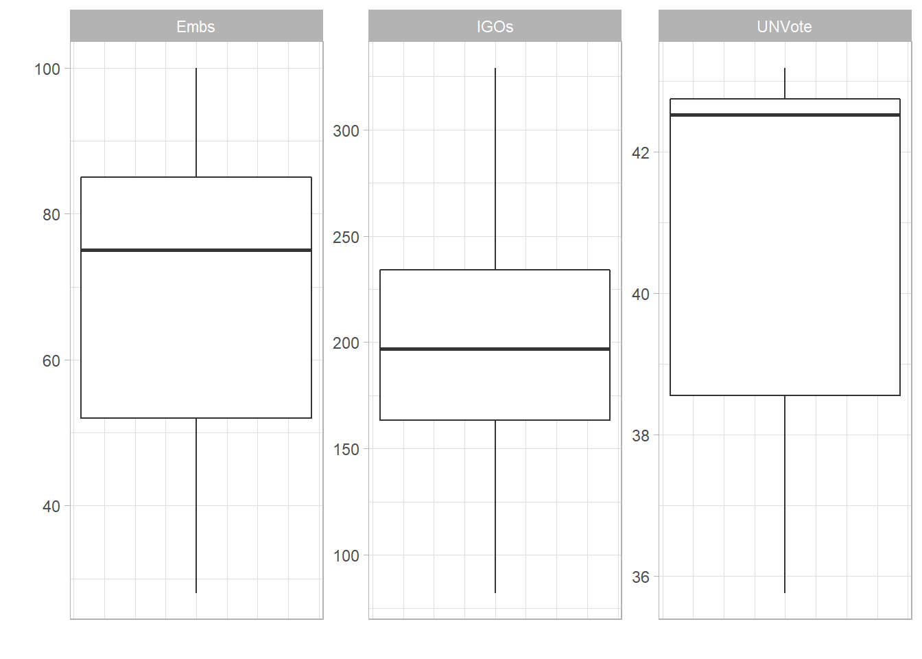
iplotIndDist(ASEM, dset = "Raw", icodes = "Renew", ptype = "Violin")Barcharts:
iplotBar(ASEM, dset = "Raw", isel = "Embs", usel = "SGP")iplotBar(ASEM, dset = "Aggregated", isel = "Conn", aglev = 3, stack_children = TRUE)Maps:
iplotMap(ASEM, dset = "Aggregated", isel = "Conn")…And many more!
Multivariate analysis
Analysing a composite indicator is streamlined in COINr by dedicated functions and plots which perform correlation analysis and PCA.
Any aggregation level (and subset thereof) can be correlated and visualised against any other:
plotCorr(ASEM, dset = "Aggregated", aglevs = c(1,2), showvals = T)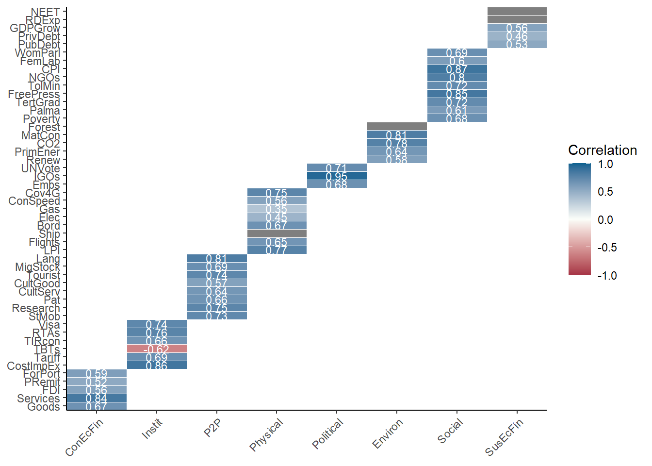
By default in-group correlations are highlighted, but the full correlation matrix can be displayed.
Multi-level correlation tables help to show weak or negatively correlated indicators with each parent level:
plotCorr(ASEM, dset = "Aggregated", aglevs = c(1,2), showvals = T, withparent = "family",
         flagcolours = TRUE)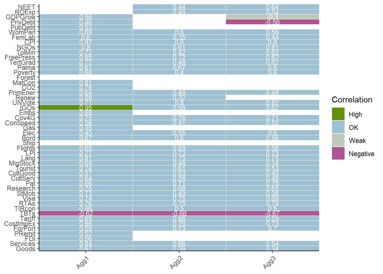
Interactive correlation maps are good for html documents:
iplotCorr(ASEM, aglevs = c(1,2), showvals = F, flagcolours = F)COINr has bindings to base PCA functions, and can give plots for any aggregation group:
library(ggbiplot)
PCAres <- getPCA(ASEM, dset = "Aggregated", aglev = 2, out2 = "list")
ggbiplot(PCAres$PCAresults$Conn$PCAres,
         labels = ASEM$Data$Aggregated$UnitCode,
         groups = ASEM$Data$Aggregated$Group_EurAsia)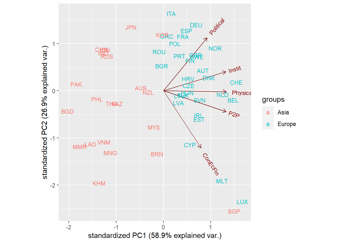
Treat data and visualise
COINr comes with a flexible set of data treatment options, including:
- Winsorisation of high and/or low values up to thresholds
- Log transformations
- Scaled log transformations
- Box-Cox transformations
Treatment can be applied to all indicators or specified individually for each. Treated and untreated data can compared using an inbuilt app.
ASEM <- treat(ASEM, dset = "Denominated")

indDash(ASEM)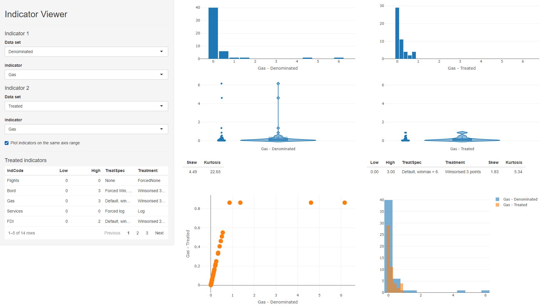
indDash screenshot
Full global sensitivity analysis
COINr calculates rank distributions for each unit, confidence intervals, and a full global sensitivity analysis which gives sensitivity indices for each input assumption. A wide range of assumptions can be varied, from weights to normalisation methods, winsorisation limits, and many more.
# plot bar chart
plotSA(SAresults, ptype = "box")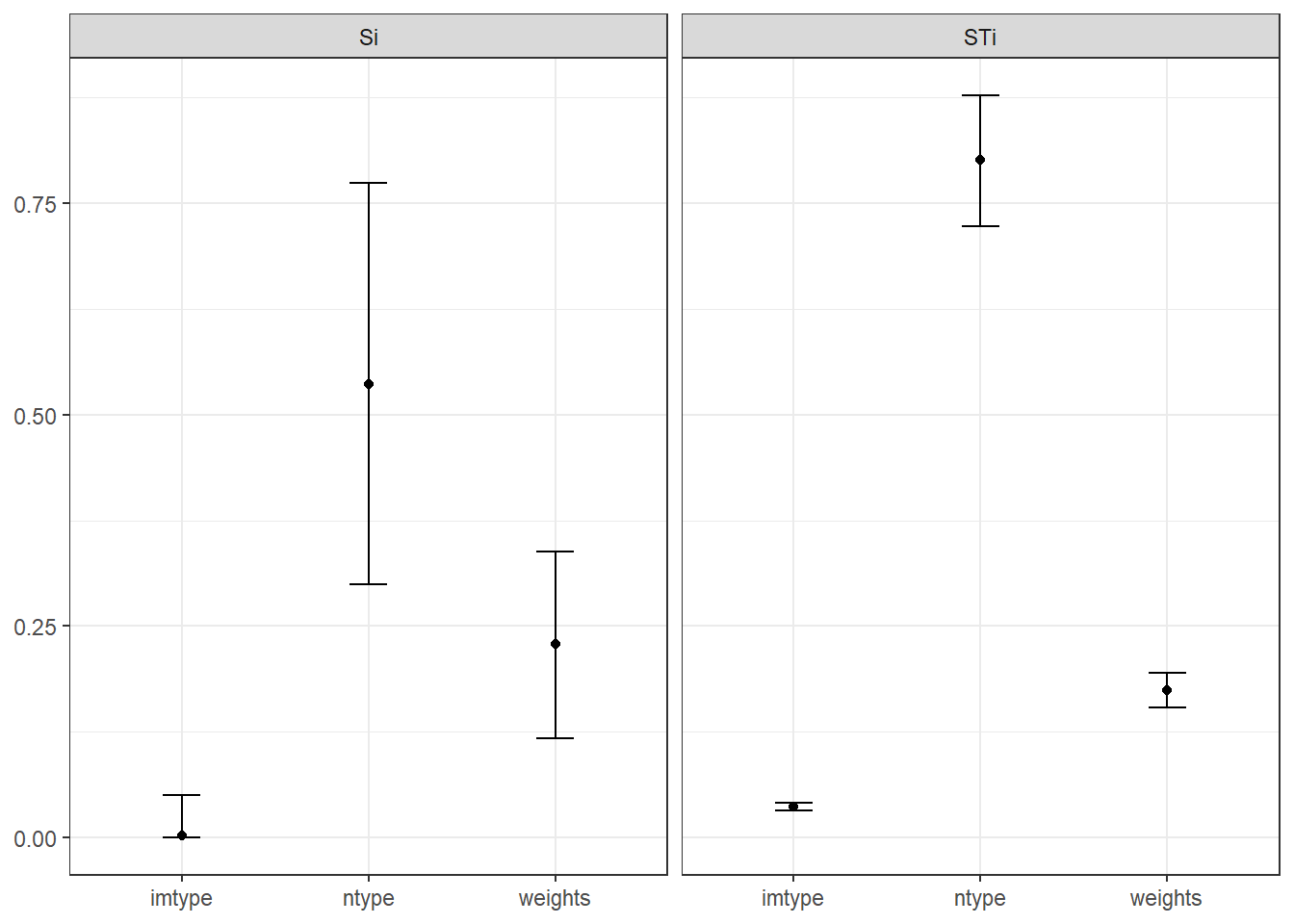
Tweak your weights
Weights can be adjusted via automatic weight optimisation, PCA, or manually. Manual weight adjustments are made easier by a built in reweighting app called rew8r(). This is currently being tweaked and is out of action, but would look like this:
rew8r(ASEM)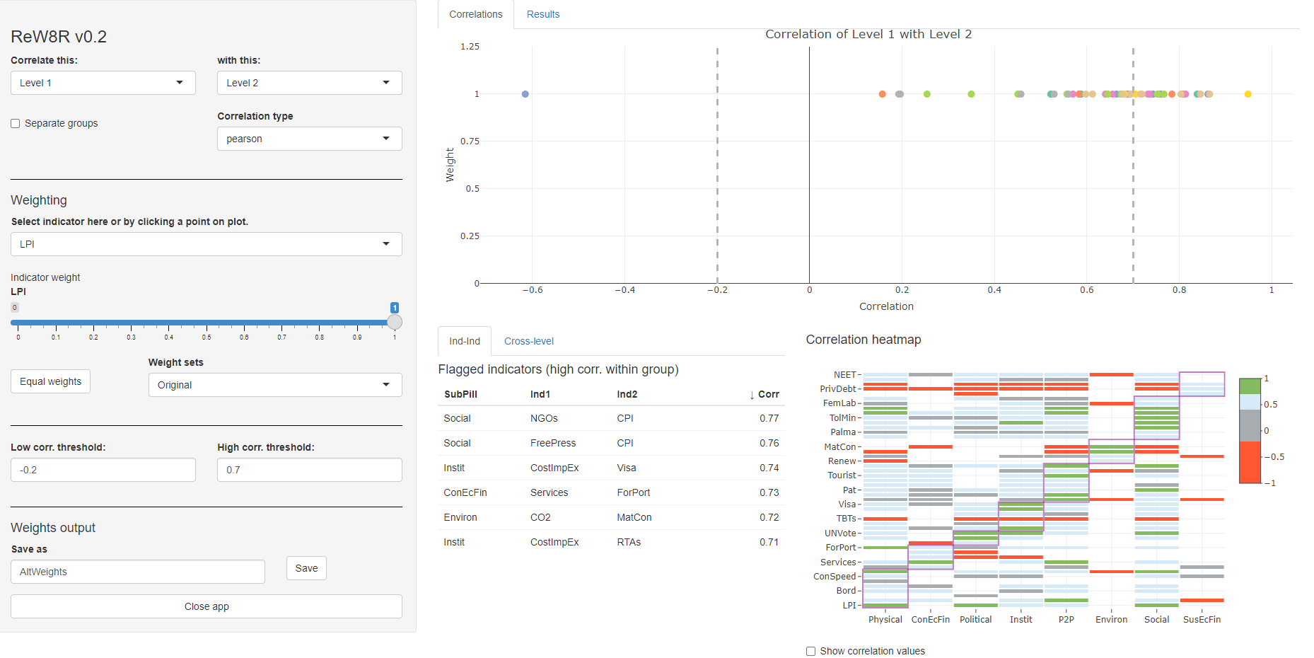
rew8r() screenshot
Fast prototype results dashboard
Results can be quickly visualised in an interactive Shiny app. This is not a substitute for a dedicated web portal, but can be a fast first exploration of the results. The app includes tables, unit comparisons, maps and bar charts. Here’s a separate example of a radar chart comparison:
iplotRadar(ASEM, dset = "Aggregated", usel = c("CHN", "DEU"), isel = "Conn", aglev = 2, addstat = "groupmean",
statgroup = "Group_GDP", statgroup_name = "GDP")And a screenshot of the full app…
resultsDash(ASEM)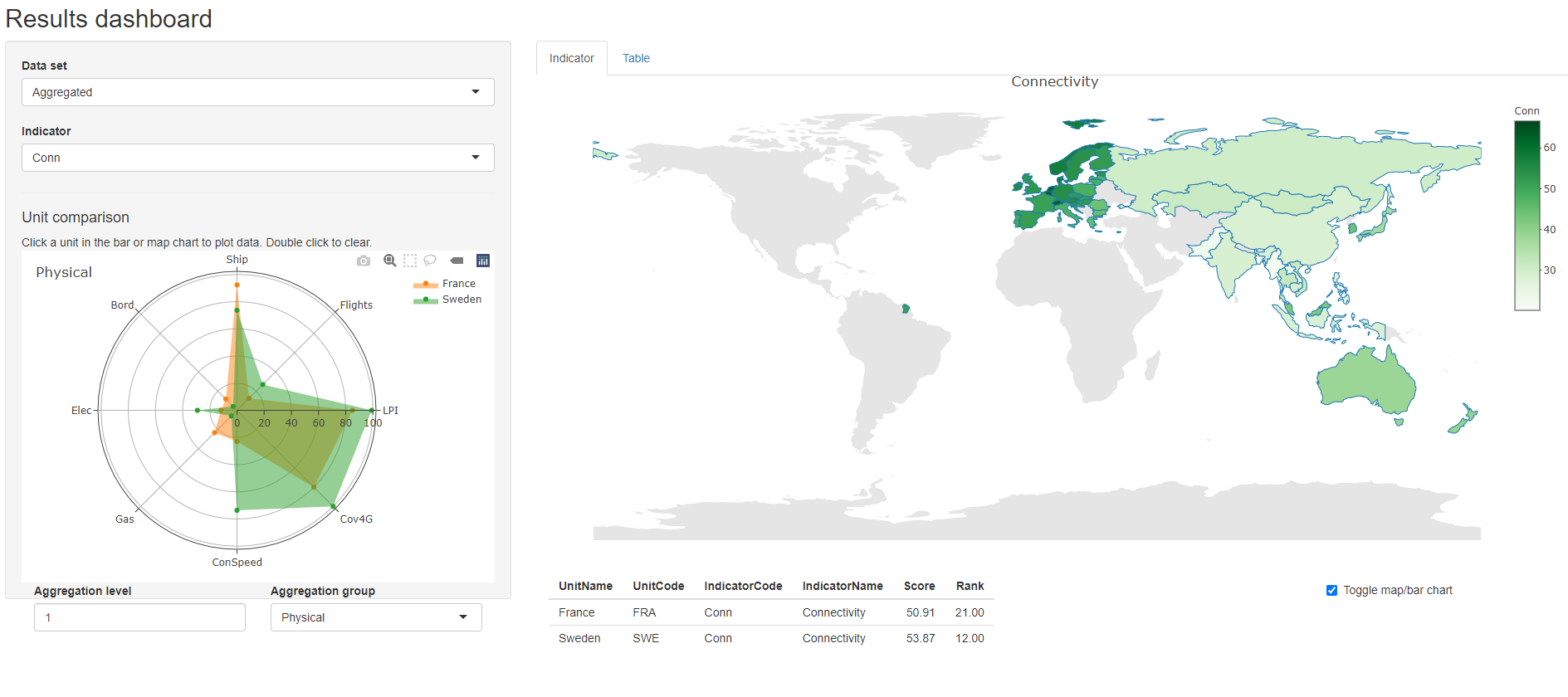
resultsDash screenshot
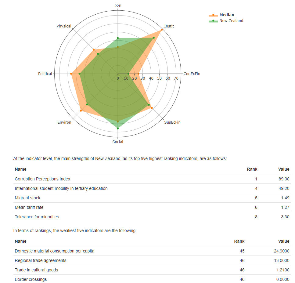
Automatic and customisable unit reports
COINr has a function which calls an R Markdown template, and generates customisable unit reports for any (or all) units. This can be output in Word, pdf, or html format.
getUnitReport(ASEM, usel = "ITA", out_type = ".docx")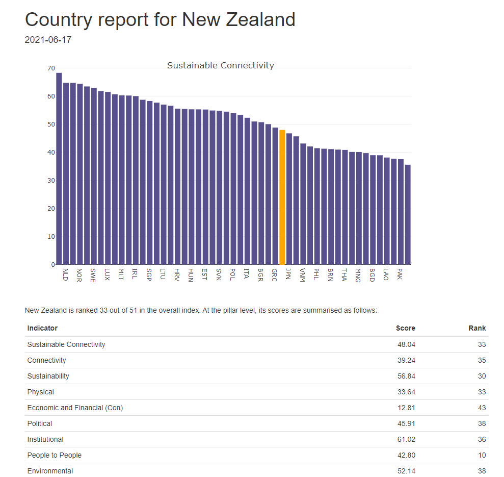
Compare versions
To adjust and compare versions of COINs, we simply:
- Copy the COIN
- Adjust the index methodology or data by editing the
.$Methodfolder and/or the underlying data - Regenerate the results
- Compare alternatives
# Make a copy
ASEMAltNorm <- ASEM

# Edit .$Method
ASEMAltNorm$Method$normalise$ntype <- "borda"

# Regenerate
ASEMAltNorm <- regen(ASEMAltNorm, quietly = TRUE)
We now make a comparison table:
compTable(ASEM, ASEMAltNorm, dset = "Aggregated", isel = "Index") #%>%## UnitCode UnitName RankCOIN1 RankCOIN2 RankChange AbsRankChange
## 43 PRT Portugal 27 16 11 11
## 29 LAO Lao PDR 48 39 9 9
## 33 MLT Malta 10 19 -9 9
## 14 EST Estonia 22 15 7 7
## 21 IDN Indonesia 43 49 -6 6
## 13 ESP Spain 19 24 -5 5
## 19 HRV Croatia 18 23 -5 5
## 17 GBR United Kingdom 15 11 4 4
## 30 LTU Lithuania 16 12 4 4
## 35 MNG Mongolia 44 48 -4 4
## 41 PHL Philippines 38 42 -4 4
## 46 SGP Singapore 14 18 -4 4
## 32 LVA Latvia 23 20 3 3
## 40 PAK Pakistan 50 47 3 3
## 4 BGD Bangladesh 46 44 2 2
## 8 CHN China 49 51 -2 2
## 20 HUN Hungary 20 22 -2 2
## 23 IRL Ireland 12 14 -2 2
## 25 JPN Japan 34 32 2 2
## 26 KAZ Kazakhstan 47 45 2 2
## 28 KOR Korea 31 33 -2 2
## 31 LUX Luxembourg 8 10 -2 2
## 37 NLD Netherlands 2 4 -2 2
## 47 SVK Slovakia 24 26 -2 2
## 48 SVN Slovenia 11 9 2 2
## 3 BEL Belgium 5 6 -1 1
## 5 BGR Bulgaria 30 29 1 1
## 9 CYP Cyprus 29 30 -1 1
## 11 DEU Germany 9 8 1 1
## 12 DNK Denmark 3 2 1 1
## 18 GRC Greece 32 31 1 1
## 22 IND India 45 46 -1 1
## 27 KHM Cambodia 37 36 1 1
## 36 MYS Malaysia 39 38 1 1
## 38 NOR Norway 4 3 1 1
## 39 NZL New Zealand 33 34 -1 1
## 42 POL Poland 26 27 -1 1
## 45 RUS Russian Federation 51 50 1 1
## 49 SWE Sweden 6 5 1 1
## 50 THA Thailand 42 43 -1 1
## 51 VNM Vietnam 36 37 -1 1
## 1 AUS Australia 35 35 0 0
## 2 AUT Austria 7 7 0 0
## 6 BRN Brunei Darussalam 40 40 0 0
## 7 CHE Switzerland 1 1 0 0
## 10 CZE Czech Republic 17 17 0 0
## 15 FIN Finland 13 13 0 0
## 16 FRA France 21 21 0 0
## 24 ITA Italy 28 28 0 0
## 34 MMR Myanmar 41 41 0 0
## 44 ROU Romania 25 25 0 0 #head(10) %>%
#knitr::kable()
Import and export
While you can get your data in and out of R in any way you want with R’s myriad packages, COINr has a couple of handy interfaces.
- The
coin_2excel()function writes all data, analysis and results to a single Excel workbook in one command. - The
COINToolIn()function reads a COIN Tool workbook and automatically imports everything into COINr.